Matlab Script to Plot the Magnitude and Phase of the Continuous Complex Function

Introduction to Bode Plot Matlab

An American engineer Hendrick Bode was the inventor of the Bode plot who worked at Bell Labs in the 1930s. Bode plot graphs the frequency response of a linear time-invariant (LTI) system. The amplitude and phase of both of the LTI systems are plotted against the frequency.  A logarithmic scale is used for frequency and as well as amplitude, which is measured in decibels (dB). The Bode plot is popular with control system engineers because it lets them achieve better-closed loop system performance by graphically shaping the open-loop frequency response using clear and easy to understand rules. To easily see the gain margin and phase margin of the control system, engineers can use a bode plot. In this topic, we are going to learn about the Bode Plot Matlab.

Syntax

The syntax for bode plot Matlab is as shown below:-

bode (TF)

How to do Bode Plot Matlab?

In Matlab for a bode plot, the bode inbuilt function is available. For using these inbuilt bode function, we need to create one transfer function on a Matlab; for that, we can use a tf inbuilt function which can be available on Matlab.

Let us see how we used these function to display the bode plot. Firstly, bode plot Matlab is nothing but plot a graph of magnitude and phase over a frequency. For that, first, we need to create one transfer function. For creating a transfer function, we need to know the numerator and denominator coefficients of that transfer function; we create the transfer function in two ways. The ways are as follows:-

1. num1= [100] ;

den1 = [1 30] ;

TF1 = tf(num1 , den1)

Firstly, we can take two variables to store the numerator and denominator coefficients, and then we just pass that two variables on the tf function, and that a comma separates two variables.

2. H = tf([30 300],[1 3 50])

In the tf function, we take two square brackets; in the first square brackets, we write the coefficients of the numerator (order s^4, s^3……, s, constant), and in the second square brackets, we write coefficients of the denominator (order s^4, s^3……, s, constant). The comma separates these two square brackets. Then use the bode function in brackets the variable which is assigned for the transfer function.

Examples

Here are the following examples mention below

Example #1

Let us consider one example for a real pole; in this example, we take one transfer function for that we create two variables'num1' and 'den1', respectively. The variable 'num1' contains the coefficients of the numerator for the transfer function, and variable 'den1' stores the coefficients of the denominator for the transfer function. The tf function generates a transfer function for given coefficients of 'num1' and 'den1' variables on Matlab. Then using two variables of transfer function 'num1' and 'den1', we can display the transfer function and stored it in variable 'TF1'.Then use the bode function in brackets the variable which is assigned for transfer function 'TF1'.

Code:

clc;
clear all;
close all;
num1= [ 100 ];
den1 = [ 1 30 ];
disp ('Transfer function :-  ');
TF1= tf (num1 , den1)
bode (TF1)

Output:

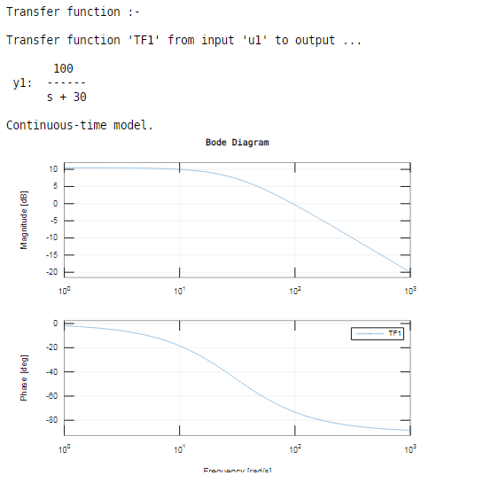
As we have seen, the result bode inbuilt function plot both the graph magnitude in dB and phase in degree over the frequency domain.

Example #2

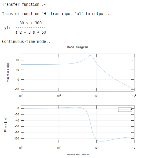
Let us see one more example related to bode plot Matlab for a complex conjugate pole.

In this example, we can take the above transfer function for a bode plot. We create the above transfer function on Matlab by using the tf inbuilt function. In tf function, we assign the coefficients of the above transfer function; in tf function, we take two square brackets, in first square brackets, we write the coefficients of numerator for the above transfer function (order s^4,s^3……, s, constant) and in second square brackets, we write coefficients of the denominator for above transfer function (order s^4,s^3……, s, constant). The comma separates these two square brackets. Then we use the bode function in brackets; we assign the variable which is used to generate a transfer function.

Code:

clc;
clear all;
close all;
disp ('Transfer function :-  ');
H = tf([30 300],[1 3 50])
bode ( H )

Output:

Example #3

Let us consider another one example related to bode plot Matlab; in this example, we compute the magnitude and phase response of the SISO ( Single Input Single Output ) system using a bode plot. First, we generate the transfer function and then use the bode function in brackets the variable which is assigned for transfer function ' H1 '. The bode takes a frequency based on system dynamic if we cannot specify the frequencies.

Code:

clc;
clear all;
close all;
disp ('Transfer function :-  ');
H1 = tf([1 10],[1 1 2 50])
[mag1, phase1, wout1]=bode (H1);                                                                            size(mag1)
length(wout1)

Output:

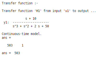
As we have seen in the result, the first two dimensions of mag1 and phase1 are one because the given system is the SISO system, and the third dimension (wout1) that is nothing but the number of frequencies.

Conclusion

In this article, we saw the concept of bode plot Matlab, firstly we understood the basic concept and definition of bode plot what exactly is bode plot Matlab and also we saw the syntax and how exactly bode plot used on Matlab and seen the resultant graphs of bode plots on Matlab that is magnitude and phase graph.

Recommended Articles

This is a guide to Bode Plot Matlab. Here we discuss How to do Bode Plot Matlab and Examples along with the codes and outputs. You may also have a look at the following articles to learn more –

1. Matlab Sort
2. Matlab fwrite
3. Matlab Syms
4. Convolution Matlab

teegardensone1962.blogspot.com

Source: https://www.educba.com/bode-plot-matlab/